Reading the HydroSOS graphs
Several graph formats are displayed in the Demonstrator in order to suggest possible formats for the operational service. The different formats offer different levels of detail, allowing even sensitive data to be presented.
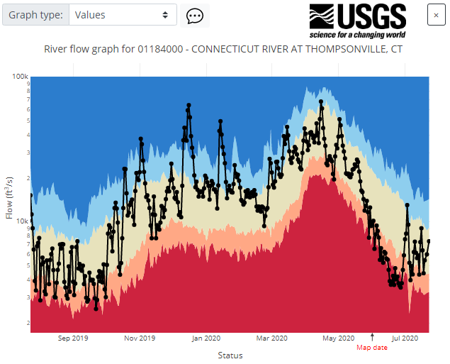
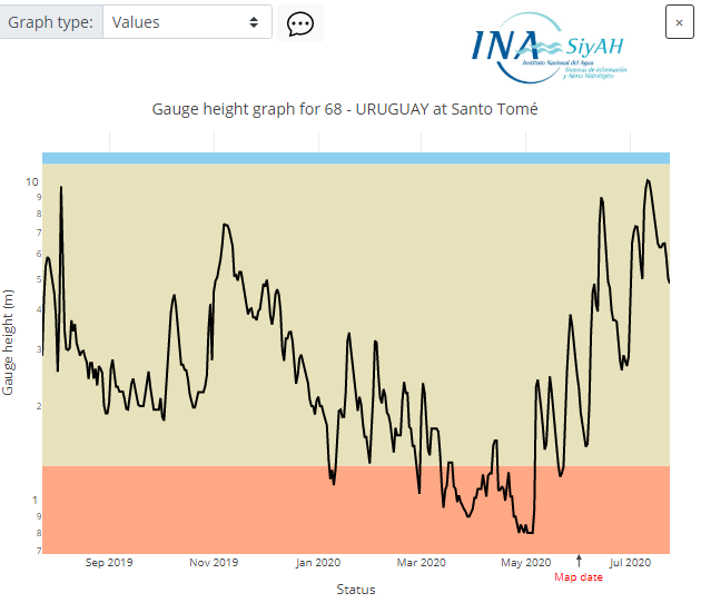
Status values graphs
Used where only status information is available, these graphs show the absolute values of the variable being shown. The background colours show the historic reference levels for each time step (e.g. above normal, normal and below normal, as shown in the USGS product) or thresholds for alerts (as shown in the Argentinian gauge height product). This enables the viewer to see if the observed flows were normal or above normal for example.
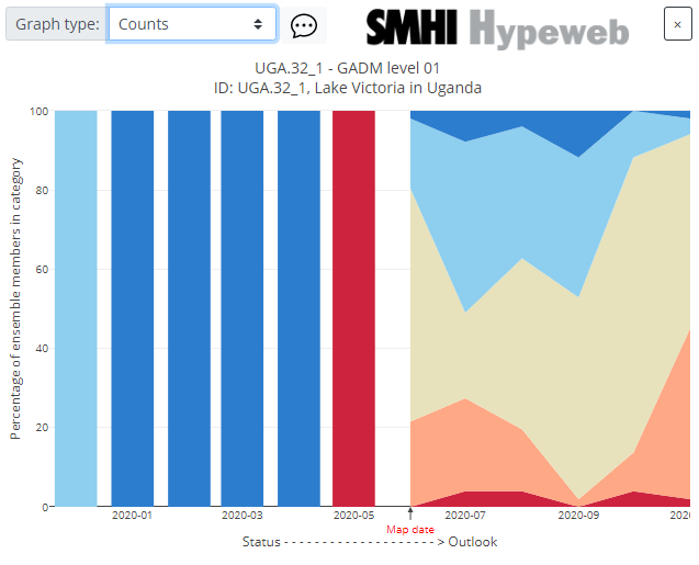
Counts graphs
The counts graphs show status/outlook information categorically, and may be useful where the underlying data is not available as part of the product.
The six bars on the left represent the status of the preceding six months. The colour represents the category (defined by long term records) the observation sits in. In the graph for example, December 2019 was classed as above normal (light blue), January through to April 2020 were classed as notably high (dark blue), and May was classed as notably low (dark red).
The outlook graph on the right shows the distribution of the forecast ensembles for the next 6 months. The height of each colour at each time step shows the percentage of ensemble members that fall into that category. In the graph for example, for June on the left hand side of the plot, 0% of ensemble members fell into the notably low (dark red) category, 21% of ensemble members fell into the below normal (orange) category, 59% in the normal (tan) category, 18% fell into the above normal (light blue) category, and 2% fell into the notably high (dark blue) category. This shows that the majority of ensemble members forecast June to be normal. By July, more ensemble members fall into the above normal category, and the blue area becomes larger. By the end of the forecast in November, on the right hand side of the graph, more of the ensemble members are in the below normal category, and the orange area is larger.
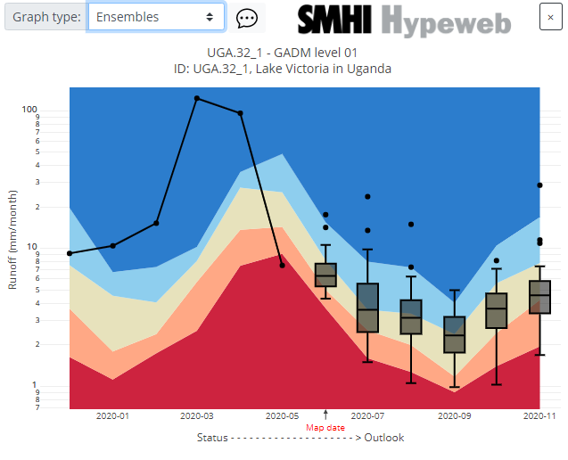
Ensembles graphs
The ensembles graph shows the status/outlook information in real units of measure, overlaid on the long-term average categories. This enables the viewer to see if the observed and forecast flows were/are normal or above normal for example.
The status part of this graph provides a line with the simulated observations from the model for six months in the run up to the forecast. The outlook part of the graph shows box plots of the forecast ensemble members.
For the SMHI global outlook, the information is given as monthly forecasts at each lead time. For the UKCEH outlook, the information is given as accumulated forecasts (e.g. the three-month forecast is an average of the one-, two- and three months' model results.
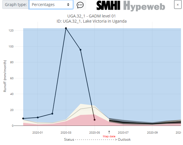
Percentiles graphs
The percentiles graph is an alternative display to the ensembles graphs. The status graph shows the observations in real units of measure, overlaid on the long-term average categories (distilled to just three categories), as well as the long-term observed monthly mean. The outlook graph shows the ensemble forecasts displayed as a shaded fan plot, giving confidence levels at the 10th–90th percentiles (light grey), and the 33rd–67th percentiles (darker grey), as well as the ensemble mean (black line).